Pandas accessors

from apsg import *

Pandas interface

To activate APSG interface for pandas you need to import it.

from apsg.pandas import pd
from apsg.pandas import gbf

We can use pandas to read and manage data. See pandas documentation for more information.

df = pd.read_csv('structures.csv')
df.head()

	site	structure	azi	inc
0	PB3	L3	113	47
1	PB3	L3	118	42
2	PB3	S1	42	79
3	PB3	S1	42	73
4	PB4	S0	195	10

We can split our dataset by type of the structure…

g = df.groupby('structure')

and select only one type…

f = g.get_group('S3')
l = g.get_group('L3')
l.head()

	site	structure	azi	inc
0	PB3	L3	113	47
1	PB3	L3	118	42
5	PB8	L3	167	17
6	PB9	L3	137	9
7	PB9	L3	147	14

Calling the accessor

Each APSG feature type has its own callable accessor directly on the DataFrame - vec, vec2, dir, fol, lin, and fault. Calling it, e.g. df.lin(), builds the corresponding FeatureSet live from whichever columns are currently configured (default azi/inc for lin/fol, x/y/z for vec, etc.) - no intermediate column is ever created. If your columns aren’t named azi/inc, reconfigure with df.lin.set_columns(azi=..., inc=...) before calling.

L3 = l.lin()
L3

L(97) lin

You can also provide name of apsg feature set.

S3 = f.fol(name="S3")
S3

S(14) S3

Calling the accessor, e.g. l.lin(), returns the live APSG feature set directly - LineationSet here - so we can use any of the APSG methods on it.

The returned FeatureSet directly exposes all APSG methods and calculations:

print('L3 R:', l.lin().R())
print('L3 kappa:', l.lin().fisher_statistics()['k'])
print('L3 var:', l.lin().var())
print('S3 R:', f.fol().R())
print('S3 kappa:', f.fol().fisher_statistics()['k'])
print('S3 var:', f.fol().var())

L3 R: L:122/8
L3 kappa: 13.750094085863328
L3 var: 0.07272677508416237
S3 R: S:161/12
S3 kappa: 17.495872632956495
S3 var: 0.05715633743905446

To calculate orientation tensor…

l.lin().ortensor()

OrientationTensor3
[[ 0.29  -0.344 -0.067]
 [-0.344  0.644  0.088]
 [-0.067  0.088  0.065]]
(S1:0.932, S2:0.29, S3:0.216)

Accessor methods

The accessor’s plot method creates a quickplot directly from the DataFrame.

l.lin.plot(label="L3")

Multiple simultaneous feature sets (wide format)

Each accessor keeps a single, stateful column configuration per DataFrame - there’s no separate config per structure type. To get multiple feature sets out of one wide-format DataFrame, reconfigure the accessor’s columns with set_columns and call it again for each structure type in turn. Here is an example of wide format data.

dfw = pd.read_csv('structures_wide.csv', dtype_backend="numpy_nullable")
dfw.head()

	site	S1_azi	S1_inc	L1_azi	L1_inc	S2_azi	S2_inc	L2_azi	L2_inc
0	PS1	<NA>	<NA>	<NA>	<NA>	<NA>	<NA>	135	11
1	PS1	69	25	<NA>	<NA>	228	70	<NA>	<NA>
2	PS1	<NA>	<NA>	<NA>	<NA>	220	59	<NA>	<NA>
3	PS1	<NA>	<NA>	<NA>	<NA>	<NA>	<NA>	<NA>	<NA>
4	PS1	<NA>	<NA>	<NA>	<NA>	<NA>	<NA>	131	11

dfw.fol.set_columns(azi="S1_azi", inc="S1_inc")
S1 = dfw.fol(name="S1")
dfw.lin.set_columns(azi="L1_azi", inc="L1_inc")
L1 = dfw.lin(name="L1")
dfw.fol.set_columns(azi="S2_azi", inc="S2_inc")
S2 = dfw.fol(name="S2")
dfw.lin.set_columns(azi="L2_azi", inc="L2_inc")
L2 = dfw.lin(name="L2")
S1, L1, S2, L2

(S(109) S1, L(6) L1, S(10) S2, L(7) L2)

Each accessor call already returns only the valid (non-NaN) rows.

GroupBy

Each accessor’s groupby(by) provides apply, transform, and aggregate methods that build the FeatureSet for each group directly from the existing columns (no intermediate column needed) and automatically recast the results back to proper extension dtypes.

The gbf module provides ready-to-use helper functions following this pattern. Note, that you have to split your data to linear and planar as statistics differs.

dfl = df[df["structure"].str.startswith("L")].copy()
dff = df[df["structure"].str.startswith("S")].copy()

Now, for example, we can compute the mean orintation per group (for vector data mean resultant is calculated, for axial data major axis of orientation tensor is used):

dfl.lin.groupby('structure').apply(gbf.mean)

structure
L1    L:299/1
L2    L:121/8
L3    L:122/8
dtype: lin

dff.fol.groupby('structure').apply(gbf.mean)

structure
S0    S:240/12
S1     S:93/13
S2    S:200/73
S3    S:163/13
dtype: fol

Functions with extra parameters pass through automatically:

dfl.lin.groupby('structure').apply(gbf.eigenlin, which=1)

structure
L1    L:208/59
L2    L:225/60
L3    L:214/18
dtype: lin

Multiple aggregate functions

You can pass multiple functions to aggregate (or agg):

dfl.lin.groupby('structure').agg([len, gbf.mean])

	len	mean
structure
L1	7	L:299/1
L2	7	L:121/8
L3	97	L:122/8

Use a list of tuples to name results when calling the same function with different parameters:

dfl.lin.groupby('structure').aggregate([
    ('major', lambda s: gbf.eigenlin(s, which=0)),
    ('intermediate', lambda s: gbf.eigenlin(s, which=1)),
    ('minor', lambda s: gbf.eigenlin(s, which=2)),
])

	major	intermediate	minor
structure
L1	L:299/1	L:208/59	L:29/31
L2	L:121/8	L:225/60	L:26/29
L3	L:122/8	L:214/18	L:10/70

Custom groupby functions

You can easily write your own functions following the same pattern. The function receives the group’s FeatureSet directly:

def vollmer_p(fs):
    """Return point index (Vollmer, 1990)."""
    return fs.ortensor().P

def vollmer_g(fs):
    """Return girdle index (Vollmer, 1990)."""
    return fs.ortensor().G

def vollmer_r(fs):
    """Return random index (Vollmer, 1990)."""
    return fs.ortensor().R


dff.fol.groupby('structure').aggregate([vollmer_p, vollmer_g, vollmer_r])

	vollmer_p	vollmer_g	vollmer_r
structure
S0	0.936789	0.007189	0.056021
S1	0.176625	0.660445	0.162930
S2	0.603624	0.107410	0.288966
S3	0.810197	0.124028	0.065774

Group transforms

Use transform to compute per-element results within each group. For example, angular distance to the group mean:

dfl['angle_to_mean'] = dfl.lin.groupby('structure').transform(gbf.angle_to_mean)
dfl[['site', 'structure', 'azi', 'inc', 'angle_to_mean']].head(10)

	site	structure	azi	inc	angle_to_mean
0	PB3	L3	113	47	39.883719
1	PB3	L3	118	42	34.354406
5	PB8	L3	167	17	45.260347
6	PB9	L3	137	9	15.366185
7	PB9	L3	147	14	25.765377
11	PB10	L3	163	9	41.038016
12	PB11	L3	294	2	12.327306
13	PB12	L3	138	17	18.531435
14	PB12	L3	140	10	18.393666
19	PB13	L3	134	1	14.171699

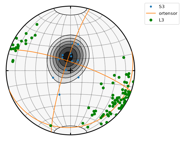
Object-oriented StereoNet

To construct stereonets with more data, you can use common APSG plotting strategy.

s = StereoNet()
s.contour(S3)
s.pole(S3, label="S3", ms=4)
pp = S3.ortensor().eigenfols()
s.great_circle(*pp, label='ortensor')
s.line(L3, label="L3", color="g")
s.show()

Fault features

The fault features could be created from columns containing orientation of fault plane, fault striation and sense of shear (+/-1).

df = pd.read_csv('mele.csv')
df.head()

	fazi	finc	lazi	linc	sense
0	94.997	79.966	119.073	79.032	-1
1	65.923	84.972	154.087	20.008	-1
2	42.354	46.152	109.786	21.778	-1
3	14.093	61.963	295.917	21.045	1
4	126.138	77.947	40.848	21.033	-1

faults = df.fault()
list(faults)[:5]

[F:95/80-119/79 R,
 F:66/85-154/20 S,
 F:42/46-110/22 R,
 F:14/62-296/21 N,
 F:126/78-41/21 D]

df[:5].fault.plot()

Materializing a real column (optional)

The accessors never create a column - that’s the point. But if you already have a FeatureSet (e.g. from linset.random_fisher(...)) and specifically want a real, materialized DataFrame column back, you can still build one directly from the matching *Array extension array class.

import numpy as np
from apsg.pandas import LinArray

random_lins = linset.random_fisher(position=lin(120, 40), kappa=30, n=10)
df2 = pd.DataFrame({'site': ['X'] * 10, 'value': np.random.rand(10)})
df2['lins'] = LinArray(random_lins.data)
df2

	site	value	lins
0	X	0.587018	L:102/45
1	X	0.939126	L:128/51
2	X	0.120167	L:159/47
3	X	0.879461	L:130/48
4	X	0.158735	L:102/47
5	X	0.734375	L:120/55
6	X	0.639178	L:90/45
7	X	0.847056	L:111/40
8	X	0.637636	L:148/54
9	X	0.829227	L:129/16