APSG tutorial - Part 5

from apsg import *

Pandas interface

To activate APSG interface for pandas you need to import it.

from apsg.pandas import pd

We can use pandas to read and manage data. See pandas documentation for more information.

df = pd.read_csv('structures.csv')
df.head()

	site	structure	azi	inc
0	PB3	L3	113	47
1	PB3	L3	118	42
2	PB3	S1	42	79
3	PB3	S1	42	73
4	PB4	S0	195	10

We can split out dataset by type of the structure…

g = df.groupby('structure')

and select only one type…

l = g.get_group('L3')
l.head()

	site	structure	azi	inc
0	PB3	L3	113	47
1	PB3	L3	118	42
5	PB8	L3	167	17
6	PB9	L3	137	9
7	PB9	L3	147	14

Before we can use APSG interface, we need to create column with APSG features. For that we can use apsg accessor and it’s methods create_vecs, create_fols, create_lins or create_faults. Each of this method accepts keyword argument name to provide name of the new column.

l = l.apsg.create_lins(name='L3')
l.head()

	site	structure	azi	inc	L3
0	PB3	L3	113	47	L:113/47
1	PB3	L3	118	42	L:118/42
5	PB8	L3	167	17	L:167/17
6	PB9	L3	137	9	L:137/9
7	PB9	L3	147	14	L:147/14

Once we create column with APSG features, we can use accessors vec, fol, lin or fault providing methods for individual feature types, e.g. to calculate resultant vector

l.lin.R()

L:122/8

or to calculate orientation tensor…

l.lin.ortensor()

OrientationTensor3
[[ 0.29  -0.344 -0.067]
 [-0.344  0.644  0.088]
 [-0.067  0.088  0.065]]
(S1:0.932, S2:0.29, S3:0.216)

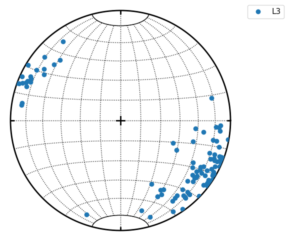
or to plot data on stereonet…

l.lin.plot(label=True)

You can also extract APSG column as FeatureSet using accessor property G

l.lin.G

L(97) L3

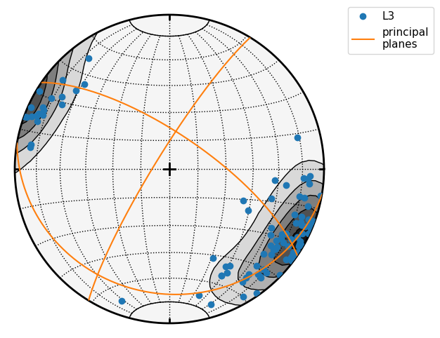
To construct stereonets with more data, you can pass stereonet object using keyword argument snet

s = StereoNet()
l.lin.contour(snet=s)
l.lin.plot(snet=s, label=True)
pp = l.lin.ortensor().eigenfols()
s.great_circle(*pp, label='principal\nplanes')
s.show()

f = g.get_group('S2').apsg.create_fols(name='S2')
f.fol.plot()

The fault features could be created from columns containing orientation of fault plane, fault striation and sense of shear (+/-1)

df = pd.read_csv('mele.csv')
df.head()

	fazi	finc	lazi	linc	sense
0	94.997	79.966	119.073	79.032	-1
1	65.923	84.972	154.087	20.008	-1
2	42.354	46.152	109.786	21.778	-1
3	14.093	61.963	295.917	21.045	1
4	126.138	77.947	40.848	21.033	-1

t = df.apsg.create_faults()
t.head()

	fazi	finc	lazi	linc	sense	faults
0	94.997	79.966	119.073	79.032	-1	F:95/80-119/79 R
1	65.923	84.972	154.087	20.008	-1	F:66/85-154/20 R
2	42.354	46.152	109.786	21.778	-1	F:42/46-110/22 R
3	14.093	61.963	295.917	21.045	1	F:14/62-296/21 N
4	126.138	77.947	40.848	21.033	-1	F:126/78-41/21 R

t[:5].fault.plot()